Hiking with Reviewer 2

This is a deep dive into my own research — the backstory behind a single line in a recently published paper and the data-driven trip down memory lane that was spurred by an innocent question from Reviewer 2. 

This research took place on Wabanaki land. I want to respectfully acknowledge the Maliseet, Micmac, Penobscot, and Passamaquoddy tribes, who have stewarded this land throughout the generations. I am certainly not the first person to devote time and energy to tracking seasonal changes on Mount Desert Island. 

This week one of my dissertation chapters, Trails-as-transects: phenology monitoring across heterogeneous microclimates in Acadia National Park, Maine, was published in the journal Ecosphere. In this project, I pulled the space-for-time trick and hiked three mountains repeatedly to collect a lot of phenology observations across diverse microclimates. The mountains in Acadia are not huge — these granite ridges roll up from the Gulf of Maine and top out at 466 m — but my transect hikes were between 4.8 km and 9.7 km each, and I wore out a pair of trail runners each season. I took to heart Richard Nelson’s advice: “There may be more to learn by climbing the same mountain a hundred times than by climbing a hundred different mountains.” 

A couple months ago, in our second round of reviews, Reviewer 2 noted, “I think that it would be useful for those wanting to replicate your transect-as-trails approach (especially land managers) to know approximately how many person hours it took to complete a transect observation, here in the main text or in the appendix.” I had a magnet (which is apparently also available as a coaster) hanging next to my desk in grad school: over a silhouette of a golden retriever with three tennis balls in its mouth, it reads: “If it’s worth doing…it’s worth overdoing.” This magnet perfectly describes my response to Reviewer 2. I sent a back-of-the-envelope estimate to my coauthors, but I couldn’t shake the feeling that the precise person hours per transect was a knowable statistic. In addition to my field notes scribbled into weatherproof notebooks, I had collected my data via fulcrum, a smartphone app that automatically recorded the time of each observation. From my cache of fulcrum csv and xlsx files, I should be able to automatically pull the time of the first and last observation of each transect. The 10.7 MB of data in my fulcrum files represented four years of field work, hours and hours on the trails, slogging through rain, snow, and sun, training field assistants, combing through patches of lowbush blueberry and mountain cranberry for the first, hidden open flower.

I became obsessed with the idea of seriously calculating person hours per transect, but I was increasingly convinced that a single number would be meaningless. I also realized that I lacked the coding chops to deal with my messy raw data: 171 files, each with 77 columns, usually containing data from a single transect, but occasionally comprising half a transect (when we had to bail due to weather) or more than one transect (when I ran ambitious double-days, or my field assistants and I split up). I turned to Porzana Solutions, and Auriel Fournier expertly helped me unlock my person hours data.Over 177 the hikes in my fulcrum files, the mean time between first and last observation is 3.51 hours.

Three and a half hours does not even begin to tell the story. This blog post is my second supplemental appendix. Here is the story of person hours per transect — the lead time, the pregnant field season, and the phenology of phenology monitoring. 

Before the first observation and after the last

There is a lead time in every transect hike. After rolling out of bed, pulling on the same old running shorts, race tshirt, and powder blue sunglasses, after packing the same handful of granola bars, dried papaya, and sharp cheddar, zipping my phone into its waterproof case, and slinging my backpack into the passenger seat, after driving to the trailhead and placing my research permit on my dashboard, there’s still a gap between the start of the fieldwork and the first official observation of the day. Especially as the summer crowds began arriving in June, I had to get out early to grab a spot at the limited parking by the north or the south end of Pemetic, or else add some extra miles from a spillover lot*. Even at the best parking spot, the approach to the Sargent South Ridge trailhead requires navigating 0.7 miles of carriage roads between the car and the trail on every hike. When I started the project in 2013, the Sequester kept Park Loop Road closed late into the spring season. For the first six weeks of fieldwork, I walked along the empty road to access Cadillac North Ridge, and Pemetic North and South Ridge.

The transect hikes were 4.8 km (Pemetic), 9.2 km (Cadillac), and 9.7 km (Sargent) up the North Ridge and down the South Ridge or vice versa (all of the mountains had uncreatively named north and south ridge trails). So at the end of a transect, I was 4.8, 9.2, or 9.7 km away from my car. I could run the carriage roads to connect the trailheads after Sargent or Pemetic (a 6.6 km run post-Sargent, and 7.2 km run post-Pemetic). From Cadillac South Ridge, a run up Route 3 to park loop road got me back to the north ridge trailhead in 10 km. Sometimes I arranged rides with friends to skip the run, and when I had funding for field assistants in 2015 and 2016 we often carpooled to drop a car at the finish line for each other. (There were some benefits to this running routine — in 2014 I won free ice cream after placing third in my age group in the Acadia Half Marathon.)

The person hours per transect statistic is limited because not every transect was a straight shot. Sometimes we had to bail 3km into a hike due to bad weather and finish the transect another day. Once, one of my field assistants took a wrong turn and recorded phenology observations on the wrong trail down Pemetic, and so I went back, retraced her steps, and picked up the right trail the next day. Once, I did a wild two-a-day and in the middle of Cadillac, I ran down the Canon Brook Trail, looped through the Pemetic transect, and then ran back up the Cadillac West Face Trail to finish Cadillac. Once, I had a friend in town and we caught a ride to the summit of Cadillac and then enjoyed the leisurely hike down the south ridge with my eight-month-old in the baby backpack.

While the time between first and last observation averaged just over 4 hours for Cadillac, 2.5 hours for Pemetic, and 3 hours and 40 minutes for Sargent, those times discount the bookends of the hikes. As much as I’m railing against the answer to my query here, the process of working with Porzana Solutions to calculate these times has been incredibly rewarding. I feel like I’m getting to know my both raw data and the tidyverse in a weirdly intimate way that goes way beyond a standard tutorial. 

The pregnant field season

In 2015 I was 17 weeks pregnant at the start of my field season. In addition to my daughter, I was also joined in the field by two field assistants. According to the Porzana analysis, I hiked less than half as many transects in 2015 (15) compared to each of the two previous years (2013: 35** hikes, 2014: 37 hikes). I actually hiked 20 transects that year — my assistants were entering the data (and getting credit for the hike in fulcrum) while we hiked together in the beginning of the season***. On my solo transects in 2015, I felt sloooooow. I averaged thirty minutes slower than 2013 and 2014 on Cadillac, 50 minutes slower on Pemetic, and 22 minutes slower on Sargent. On top of this, I was covering less ground — in 2013 and 2014 I had monitored phenology in off-trail Northeast Temperate Network plots near my transects in an effort to compare trail-side phenology with forested sites that was ultimately cut from my dissertation. In 2015, I stuck to the trails.

I remember feeling pretty terrible at the beginning of most hikes that year. I had one favorite spruce tree on the south ridge of Sargent, and I can picture myself looking up through the needles on more than one occasion from my lie-down-spot while I tried to decide if a bite of granola bar would make me feel more or less nauseous. As I climbed above treeline and into the breeze the fog of morning sickness would lift, and as I hiked downhill, my daughter would do this funny little fetus-roll and kick in a way that I interpreted to be happy.

Hiking while pregnant was hard, but it felt easier than grappling with the looming challenges of becoming a parent. I liked the hard of fieldwork, it was the kind of hard that I felt capable of conquering. I also loved being pregnant in Bar Harbor. It was my fifth field season in Acadia and I had this wonderful community of supportive colleagues and mentors at the park service and in town. I had a favorite yoga class, a favorite milkshake, a favorite iced chai and blueberry muffin spot. I also had two field assistants — my pregnancy fortuitously aligned with NSF funding! — and working with Ella and Natasha that season was great. The person hours per transect figure obscures my field assistants, folding us into each other and masking the time we spent training together on the ridges. It also hides my pregnancy in the averages. I want to recognize those extra 22-50 minutes: they were some of the best worst minutes of my PhD.

The phenology of phenology monitoring

The person hours per transect average doesn’t show the sprint finishes of June. I monitored thirty species (the paper highlights the 9 most common taxa) of spring-flowering plants. On the transect hikes, I recorded leaf out and flowering phenology. In April, this was a bit of a scavenger hunt, and I’d pour over thickets of shrub stems for the first sign of bud break, then in May I’d peek into each curled Canada mayflower leaf for flower buds. By early June, my plants had leafed out, and the flowering season was winding down. I knew the trails by heart, and the location of each focal taxa along the ridge was bright in my mental map; each transect became a point-to-point trail run between the last phenological hold outs. Did the rhodora finish flowering on Cadillac? Had the last sheep’s laurel buds opened on Pemetic? Were the blueberries beginning to ripen below Sargent’s summit?

As I followed the spring phenology, I grew faster, my calf muscles more defined, my appetite more voracious. Acadia’s steep climbs will whip you into shape. I remember in 2013 arriving in the field a month after passing my comps and feeling so sluggish after a winter of studying instead of running. In comparison, I ran hard in the winter of 2013-2014, set a personal best half marathon time in a trail race in March, and just cruised through the early season field work in 2014. Even in 2015, as I grew rounder each week, I also grew more comfortable with the trails. Hiking while pregnant became easier over the season, although I’m happy it ended when it did, because that trend was not sustainable into the third trimester. 

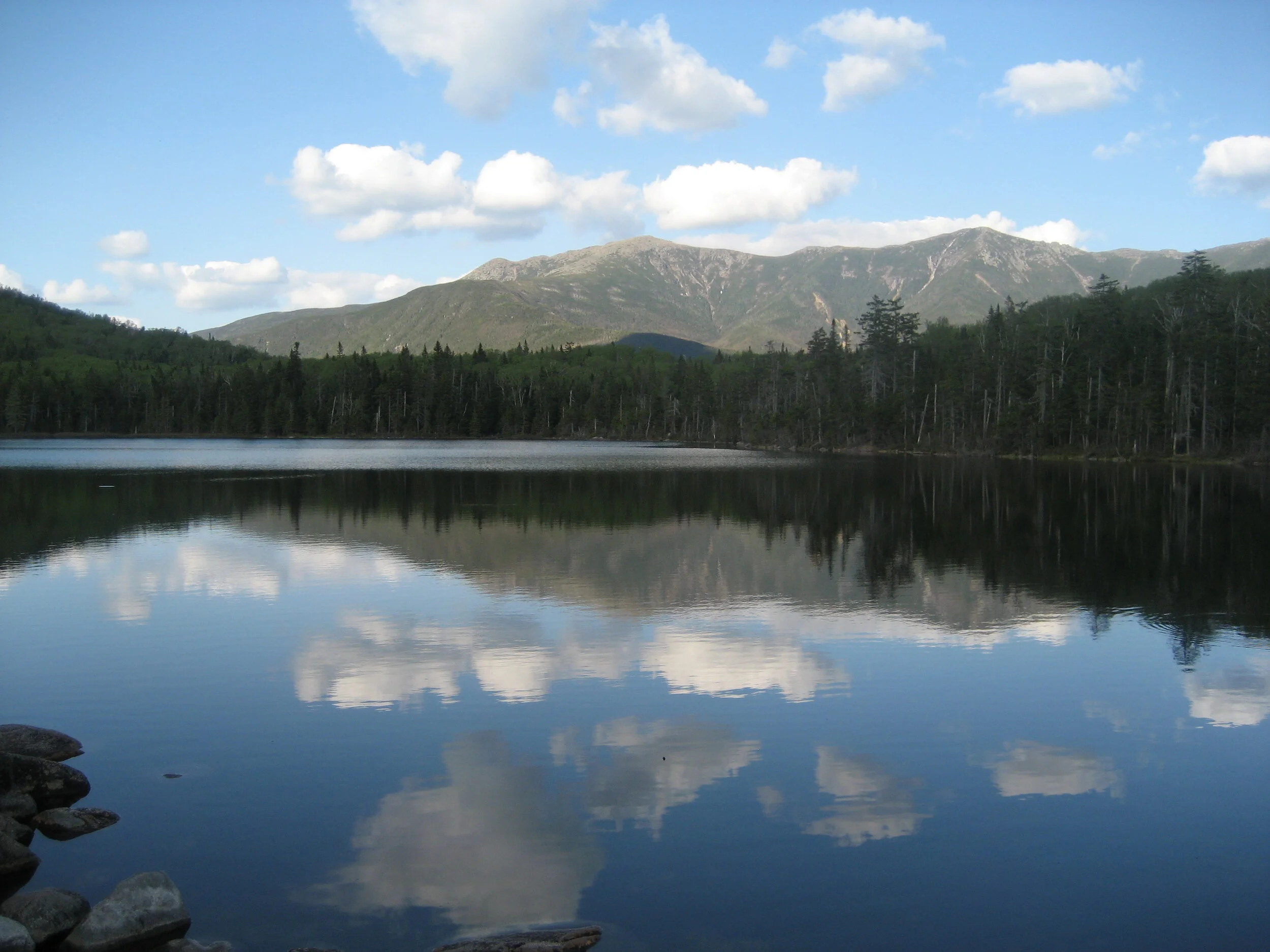
I think about Reviewer #2 and I want to ask: do you mean the person hours per transect in April? Or at the end of June? What kind of mileage were you averaging before the start of the field season? Do you have any old hamstring injuries? Tell me about your field assistants. Do you like to stop for lunch at the summit or are you an on-the-go-snacker? Did you pack a couple bucks to buy a Harbor Bar at the Cadillac souvenir shop? Are you saving your energy for the 10k run at the end of the transect? Is the National Park Service well-funded in this year’s federal budget? How do you feel about stopping for a swim in Sargent Mountain Pond?

I love these questions because each one pulls on a thread winding through my Acadia memories. I hiked upwards of 125 transects between 2013 and 2016, and now that the paper is done, I’m a little sad to be shelving the fieldnotes for good. The trail runners that I wore are long gone, my field hat fell apart, most of my baggy race tshirts carried me through my second pregnancy and suffered for it.

In the end, the idiosyncrasies of the hikes were smoothed and flattened into the sentence, “Each transect could be completed in under 6 person-hours.” This is both true and wildly circumscribed. Not unlike a well done chapter of a PhD dissertation.

*Acadia National Park actually closed the lot by the Pemetic North Ridge trailhead in 2017 and it’s now exclusively a bus stop for the island explorer, the free bus that begins running right as my season wraps up at the end of June.

**This doesn’t include hikes before I had figured out the fulcrum platform. There was "no" data on those hikes (nothing was leafing or blooming, no signs of budburst) and they only exist in my field note books.

***I hired three field assistants for this project and, concurrently, a common garden experiment. In 2014, Paul was my garden guy, but we also hiked two transects together and he hiked two solo. In 2015, Ella, Natasha, and I split the transect and garden work. Ella came back for most of the 2016 season and then I finished the two projects solo in June 2016.

Summer Reading (Part 1)

We’re rushing out of the dog days of summer and into the start of a new semester — or in my case the start of parental leave, which is a little bit like embarking on a new semester at an unknown campus and while I completed the newborn syllabus three years ago, I have this sinking feeling that I don’t even know which classes I’m enrolled in yet. Regardless, I’m reflecting on my summer reading.

Over June, July, and August, I was all in on #365papers and I have a top ten list of scientific papers from these long summer days of slow reading. Because my “semester” might start at any moment, I’m breaking this post into two parts. First up: my favorite hot-off-the-press summer reads on mountains and phenology.

On Mountains

Think globally & way into the past…

1. Iglesias, V., Whitlock, C., Krause, T.R., Baker, R.G., 2018. Past vegetation dynamics in the Yellowstone region highlight the vulnerability of mountain systems to climate change. Journal of Biogeography 45, 1768–1780. doi:10.1111/jbi.13364

Fifteen pollen records covering 16,000 years and the 80,000 km2 mountainous Greater Yellowstone Ecosystem create an incredible review of elevational patterns of vegetation change in an iconic mountainous region. In this paper, Dr. Virginia Iglesias lays out the challenges of quanitifying pollen-vegetation relationships in mountain regions (aka what I didn’t know when I proposed my postdoc research) and then pulls in a staggering amount of modern and fossil pollen data to recreate the history of Yellowstone’s dominant conifers. These are stories of both stability and rapid change through past climatic changes with conservation implications for managers facing anthropogenic climate change. My favorite line: “The current vegetation distribution is, at best, a short and rather anomalous baseline for evaluating ecological responses to future climate change.” 

2. Elsen, P.R., Monahan, W.B., Merenlender, A.M., 2018. Global patterns of protection of elevational gradients in mountain ranges. PNAS 115, 6004–6009. doi:10.1073/pnas.1720141115

This study has it all: mountain biodiversity love, protected area planning, big data analysis, and beautifully designed maps of “elevational protection” across the globe. Full disclosure: Dr. Paul Elsen is a fellow Smith Fellow and I also got to see this paper as a speed talk at the North American Congress for Conservation Biology in July. The bottom line is this: when you zoom out, most of the world’s mountain ranges are narrowly protected — we need conservation across elevation gradients to effectively protect species under climate change. 

On Phenology 

Wherever you get your phenology data (maybe from TV?) scientists are asking some really interesting questions about community composition, temporal dynamics, and the implications of climate change on interspecific relationships…

3. Carter, S.K., Saenz, D., Rudolf, V.H.W., 2018. Shifts in phenological distributions reshape interaction potential in natural communities. Ecology Letters 30, 133–9. doi:10.1111/ele.13081

Amphibian breeding phenology is not the kind of phenology that I study — I don’t install recorders at ponds to capture EPs of overnight breeding calls, I don’t log hours listening to the audio to identify twelve different amphibian species and record the number of individuals per species calling during each recording session, and I certainly have not done this tirelessly for fifteen years. But I’m so glad that Dr. Shannon Carter and her colleagues did because their ingenuous analysis of changes in the timing of calling between pairs of amphibian species has huge implications for how we — plant phenology people included! — study phenological mismatch. The overlap (or "phenological distributions") of amphibian breeding calls has shifted in weird and non-uniform ways, and metrics like ‘first day of calling’ or ‘median call date’ don’t capture these changes well. This is just a great analysis of a grinder ball dataset (8 ponds in Northeast Texas, monitored consistently over 15 years) which opens up a window to these big questions — How do we monitor phenology? What information do we need to know that temporal mismatch is occurring?

4. De Frenne, P., Van Langenhove, L., Van Driessche, A., Bertrand, C., Verheyen, K., Vangansbeke, P., 2018. Using archived television video footage to quantify phenology responses to climate change. Methods Ecol Evol 149, 1791–9. doi:10.1111/2041-210X.13024

Dr. Pieter De Frenne and his coauthors have received tons of press coverage (best sub-headline: "ignore the lycra—look at the flowers") for this incredibly photogenic work. They basically watched 200 hours of TV (old coverage of the Tour of Flanders), justified this as “research” by grabbing screen shots of 46 shrubs and trees from along the cycling course, and found surprisingly strong advances in the timing of spring leaf out and flowering in these plants over the years. This is, on one level, the opposite of Carter et al listening to frog calls for fifteen years — the phenology monitoring here is opportunistic and there is only a single metric each year (what was happening on the day they filmed the Tour). But as De Frenne points out at the end of the paper: “Probably the most promising way forward for phenology research is to better integrate all types of phenology data…observational time series, experimental manipulations of climate, herbarium records, historical surveys of vegetation, historical maps, repeat photographs and other, yet unexploited, sources such as television video footage from broadcast archives.” 

5. Winkler, D.E., Butz, R.J., Germino, M.J., Reinhardt, K., Kueppers, L.M., 2018. Snowmelt Timing Regulates Community Composition, Phenology, and Physiological Performance of Alpine Plants. Front. Plant Sci. 9, 631–13. doi:10.3389/fpls.2018.01140 

Dr. Daniel Winkler, PLoS ESA Reporting Fellow 2016, tweeted out his new paper in July and he had me at “community composition, phenology, and physiological performance of alpine plants.” My “alpine-ish” communities include true alpine on Katahdin, but also Cadillac Mountain in Acadia, which is a whopping 1,530’ and more accurately described as ‘Northern Appalachian-Acadian Rocky Heath Outcrop’ by NatureServe. I’m definitely interested in the differences between alpine-restricted species and wide-ranging species. Winkler’s team recorded species diversity, flowering phenology, and physiological measurements including gas exchange, net CO2 assimilation, and stomatal conductance across plots along an elevation and aspect gradient in the Colorado Rockies. Two results jumped out at me: the alpine-specialists displayed less flexible flowering phenologies than the wide-ranging species, but there were not strong differences between these groups in physiology. This is the kind of paper that inspires mad grant writing — I'm interested but skeptical, will this hold up in my pet region/ecosystem/study system? I want to replicate this kind of research in the Northeast — and across a gradient of sites where phenology is tied to snowmelt (true alpine areas of Katahdin and the Presidential range), and where the two are (I think) decoupled (Cadillac Mountain). Winkler and I wrote a blog post together in 2016, I think I can convince him to collaborate on a larger scale — and get him to New England! 

Bonus “Reads”

Recent podcast episodes tangentially related to recent blogging

• This American Life covers The Feather Thief. My review of the book.

• Outside/In reports on underrepresentation in outdoor gear (aka 'shrink it and pink it' does not make women happy shoppers, especially when we can't find our sizes, preferred styles, or performance level). This touches on some of the same themes — inclusion & diversity in the outdoors — as my response to “Have Ecologists Lost Their Senses? Walking and Reflection as Ecological Method”

An Epic Joshua Tree Roadtrip & the Reproductive Ecology of an Iconic Southwest Plant

Think of your most amazing four-state roadtrip. How much data did you collect between stops at Disney Land and the hotel pool? Did you stargaze in the Mojave Desert or were you too exhausted after a day of running transects through Joshua Tree National Park? Did you look at the famous Joshua trees with wonder and awe, or did you keep your head down and count individual flowers on these episodic bloomers then hastily move on to the next site to keep tallying reproductive metrics? Did you come home to your computer and upload slideshows of vacation snapshots or did you immediately begin writing up notes like:

Despite its prominence in plant communities of the Mojave Desert, surprisingly little has been published on its reproductive and structural ecology. The majority of research on Joshua tree has focused on its highly coevolved pollination relationship with the Yucca moth. Outside its pollination biology only a few studies have been published on its reproductive ecology.

Thanks to one amazing roadtrip — with a little help from Disney World and Denny’s — new research is shedding some light on patterns of flowering, fruit production, and stand structure of Joshua trees across the Mojave Desert. I did not realize how “hashtag blessed” my own phenology research was until I read Samuel St. Clair and Joshua Hoines’ new PLoS ONE paper on the reproductive ecology of Joshua trees.

My research is a steady annual routine: I study flowering in plant populations that consistently bloom every spring when I arrive in Maine to record them. St. Clair does not have this luxury with Joshua trees — he writes: “episodic blooms make it hard to anticipate a study of its reproduction.” Early in 2013, St. Clair saw Joshua trees blooming at his field sites and called around — the trees seemed to be blooming across their range, he “even heard reports of blooming in Las Vegas and Phoenix yards.” As it became clear that 2013 was a rare opportunity to study reproductive ecology for an unpredictable study organism, St. Clair jumped to take advantage.

“Obviously there was little time to spare. I mapped out a range wide survey of populations, put a travel map together and booked hotels. Took my two sons out of school (ages 10 and 9) for field help in early May and promised them a stop at the Adventure Dome in Las Vegas and a day at Disneyland. We jumped in our car and were off.” St. Clair, a professor at BYU, and Hoines, at the National Park Service, split the fieldwork and covered ten study sites across four states in May and June 2013.

At each site they collected data on the population characteristics (population density, tree height, trunk diameter) and reproduction (number of inflorescences and total fruits, percent of trees in bloom, fruit mass, seed number) of 120 Joshua trees. That’s 1200 trees — from 60 100-meter transects! — in under two months. St. Clair shared some memorable moments, “A grasshopper outbreak at Lytle Rach that had the boys in tears, Kids eat free at Denny’s at least 4 or 5 nights and Disney Land was awesome. The boys still talk about the trip fondly.” The opportunistic rush for reproductive data revealed interesting patterns across the climate gradient of the Joshua tree’s range. At warmer sites, the Joshua trees produced more flowers and seeds, but stand density was lower, while at cooler sites, there were more Joshua trees but fewer flowers and fruit per tree. So while warming temperatures may be good news for reproductive success, the establishment of new Joshua trees seems constrained by warmer temperatures. I asked St. Clair what these results meant for Joshua trees facing climate change. “I think the bigger limitations moving forward will probably be in the seedling establishment and recruitment phases of development.  The fruiting success suggests that the pollinator populations are intact which is good—we’ve see pollination failure due to a lack of yucca moth in populations of Banana Yucca in a recent paper we published.” 

The future of Joshua trees in Joshua Tree National Park is not just a concern for scientists. The official twitter account of the Park (@JoshuaTreeNPS) garned five minutes of fame last November when they began tweeting about the potential effects of climate change on the park’s biodiversity. Secretary of the Interior Zinke apparently reprimanded the Joshua Tree National Park superintendant for these social media science lessons.The idea that a national park should be dissuaded from sharing research on the natural and cultural resources — including, the namesake of that park — with visitors and general public is truly absurd.

I think this means that it is our responsibility to tweet out the results and implications of St Clair and Hoines’ new paper and continue the conversation that @JoshuaTreeNPS started. 

Reference:

St. Clair SB, Hoines J (2018) Reproductive ecology and stand structure of Joshua tree forests across climate gradients of the Mojave Desert. PLoS ONE 13(2): e0193248. https://doi.org/10.1371/journal.pone.0193248

A Little Light Reading

As the leaves fall this October and the canopies bare their skeletal limbs, there’s suddenly more light filtering across the riverside trails in Maine and I’m wearing sunglasses on runs where I used to be totally engulfed in the shade. It’s hot toddy season, pumpkin spice season, submit-your-GRFP season. When the weather finally chills we’ll get into ugly sweater season, rush-to-take-family-photos-for-a-holiday-cards season, and grading-endless-finals season. Culturally, we humans divide the year into more than just autumn-winter-spring-fall. A recent PLOS ONE paper makes the case that understory plants probably do this too.

Janice Hudson and her coauthors explored the seasonal dynamics of sunlight in a temperate deciduous forest and the ecology of the common shade-tolerant shrub, spicebush. They were inspired, in part, by a relatively obscure 1977 Ecological Monographs paper* with the unassuming title “The Distribution of Solar Radiation within a Deciduous Forest,” in which the authors, Boyd A. Hutchison and Detlef R. Matt, outline the concept of phenoseasons.  

Get ready to update your calendars — the seven phenoseasons for life under a forest canopy are: winter leafless, spring leafless, spring leafing, summer leafing, summer fully-leafed, autumnal fully-leafed, autumnal partially-leafed. I only wish that Hutchison and Matt had dined with Tolkien. Imagine the invitation: “Let’s meet for second breakfast to celebrate the end of spring leafless.” [Insert ent joke here.] Hudson was interested in how changes in light availability affected understory plants like spicebush. As Hudson explains “broadly, this study was an attempt to better understand the pre-existing conditions of the forest…[are] light conditions...a controlling factor in the distribution and presence of plant species?” The phenoseason construct hasn’t taken off in ecology and the annual cycle of subcanopy light exposure is not well understood. Hudson and her coauthors stumbled on Hutchinson and Matt while working on a literature review, but the idea of phenoseasons — now update-able with a high-tech piece of equipment called line quantum sensors — seemed ecologically intriguing. Hudson’s background is in eco-hydrology and the link between seasonal changes in light and phenology had immediate implications for her. She wanted to know “how understory plants acclimate…[and] plant contributions to nutrient and water cycling during individual phenoseasons, and yet, the literature on the subject of phenoseasons is scant.”

Hudson’s team combined a year of intense field measurements with experimentally manipulated light conditions in growth chambers to explore light intensity through the phenoseasons. At Fair Hill Natural Resource Management Area in Maryland, Hudson and her team carried a light sensor through the forest of American beech and yellow poplar trees to measure light conditions above, within, and under the spicebush canopy, compiling over 4,500 measurements in a year across 26 sites (25 in the forest, one open area just outside the forest for comparison). 

When Hudson talks about light, she talks about photosynthetically active radiation (PAR) and, for this study, subcanopy photosynthetic photon flux density (PPFD), which is a measure of PAR. Unsurprisingly, the highest PPFD values under the beech and poplar canopy occur in spring leafing — the days are growing longer, the northern hemisphere is tilted toward the Sun, the trees are still mostly bare. During summer leafing, the subcanopy PPFD values drop, and continue to decrease into summer and autumnal fully-leafed, before a slight bump for the autumnal partially-leafed phenoseason. In a nod to Hutchison and Matt, Hudson recreates their 1977 figure mapping the contours of PPFD through the year at different canopy levels with her own data. It’s the scientific equivalent of siblings re-staging family photos as adults.

But what does it mean to be a spicebush living in the light environment depicted in these figures? In general, Hudson found that there’s almost 10 times more subcanopy light available during the leafless seasons than the leafing and leafed seasons. During the leafing and leafed seasons there are high-energy sun flecks and hot spots — think of a sun-dappled forest floor — which contribute to the variability of light measurements throughout the phenoseasons. But, mostly the understory species must make proverbial hay (read: Germinate! Flower! Leaf out! Photosynthesize like crazy!) while the sun shines in the short leafing seasons. Even in the leafless seasons, the open site received much more PPFD than the subcanopy: the woody surfaces of the trees were intercepting plenty of winter and early spring light.

The spicebush plants in the field and in the growth chambers grew best under the highest PPFD conditions found in the Maryland woods. This is the light niche. In the growth chambers, plants that received higher PPFD conditions were actually less healthy, produced fewer leaves and less biomass. Hudson wrote a beautiful explanation of this when we emailed and I have to let this paragraph speak for itself:

We know that all organisms have an ecological sweet spot, but very rarely are all conditions ideal. Canopy species are "less limited" in the sense that they may experience some shading by neighbors but are primarily subject to changes in light due to latitude, season, and sky conditions. This "light intensity niche" is especially important for shade-adapted and shade-loving plant species when you consider spectral filtration (one way that plants "communicate" with each other and adapt growth direction and strategy) and temporal sequences of incident radiation at both long and short time scales (the timing and amount of light availability is crucial for physiological and biochemical processes for these species). It puts a sort of "ceiling" on the amount of light that is useful for the understory plant, whereas for canopy species there really isn't such a thing as too much light – their growth is primarily limited by the lower boundaries of light availability.

 Finally, this study’s implications for climate change research are quite interesting. In the decades while the ‘phenoseasons’ concept was languishing, research in phenology has taken off: the timing of seasonal events like leaf out and flowering are almost universally creeping earlier in response to warming temperatures. This advancing spring phenology has been definitively tracked in temperate deciduous forests like Hudson’s study site. As the climate changes, leafing phenoseasons may bite into the leafless phenoseasons. The density of the canopy may change as the species composition, size, and height of canopy trees changes. As Hudson wrote, these are the pre-existing conditions in the forest from the perspective of an understory species. We often think about species migrations and no-analog communities when we talk about the ecological effects of climate change: now I think I’ll imagine the reshuffling of the pre-existing conditions, and the interactions between biotic and abiotic factors that create the “ecological sweet spots” that we study. And now, as we enter the autumn leafless, I’ll soak up the sun on my unseasonably warm October runs. 

*This paper’s obscurity is not helped by the fact that the google scholar pdf link takes you to a 627-page annual report hot off the mimeograph with old-timey typer-writer kerning; Hutchison and Matt’s paper is buried in this report (just scroll to page 327), though much easier to find via JSTOR.

Common Gardens For All Your Climate Change Needs

A guest post from PLOS Ecology Reporting Fellows, Caitlin McDonough MacKenzie & Daniel E. Winkler, on research from the Ecological Society of America Scientific Meeting in Ft. Lauderdale, Florida, August 7-11, 2016. 

Experimental gardens are an old-school methodology. In perhaps the best known example in the 1930s and 1940s Clausen, Keck, and Hiesey transplanted Potentilla glandulosa across their range in the Sierras to explore the roles of environment and genetics played in determining growth form. Clausen, Keck, and Hiesey’s classic methodology of reciprocal transplanting has a contemporary application in climate change studies, whereby researchers relocate a plant (or seed) from its home and current climate to a transplant garden and new (and perhaps future) climate. Seven decades later, the Ecological Society of America’s 2016 Annual Meeting features experimental gardens that include species ranging from alpine forbs to douglas fir trees to a dune-loving annual—collected along latitudinal, elevation, and habitat gradients. 

Nicole Rafferty opened the Climate Change: Ranges & Phenology I session presenting her research on patterns of bumblebee visitation at the Rocky Mountain Biological Laboratory. As a part of this project, she installed a reciprocal transplant experiment with seeds from three elevations planted at 12 plots per elevation site. She wanted to test how alpine plant-pollinator relationships might change as plant communities experience new microclimates (for example, if a species is transplanted to a warmer site at a lower elevation). Unfortunately, the first year of this study coincided with a dry summer and low germination rates — as a result, in 2016 she switched to seedlings. In her 2015 seed study, the glacier lily seeds from mid-elevation had the lowest success in the transplants, suggesting that mid-elevation might be a barrier to plant migrations upslope for this species.  

Range shifts and phenological are also on the minds of researchers at the U.S. Forest Service. This time with an applied focus aimed at aiding land managers who will likely need to develop strategies to make Forest Service lands more resilient to climate change impacts. Sheel Bansal at the U.S. Forest Service’s Pacific Northwest Research Station and colleagues carried out a large-scale common garden study aptly named the Douglas-fire Seed-Source Movement trial. Their experiment used seeds from 60 sources throughout the species range in Washington, Oregon, and California and grew trees from each of the sources in 9 climatically-divergent field sites and also used artificial freeze experiments to test the impacts of changing environmental queues on Douglas fir cold hardiness and associated genetic linkages. They found strong differences in cold hardiness, with minimum winter temperatures and fall frosts as major predictors of cold hardiness based on seed source. Their results have important implications for the ability of species to shift their ranges by tracking climate envelopes, and further extend to land management efforts to maintain healthy forests experiencing future climates.

In the Great Lakes region, Elizabeth LaRue from the Emery Lab at the University of Colorado Boulder used a common garden to explore dispersal traits in American sea rocket (Cakile edentula var. lacustris). She knew that dispersal traits like pericarp, or seed wall, thickness and wet mass varied across the Cakile edentula range, but it was unclear if the variability was caused by environmental or genetic differences. Collecting seeds from across the range, and growing them together in a common garden isolated the role of genetic differences and revealed lower dispersal traits at the range edges. This data was used to inform species distribution models with different scenarios for starting dispersal genetics for Cakile edentula under climate change.

Kennedy Rubert-Nason in the Department of Entomology at the University of Wisconsin-Madison and his colleagues looked at the role of vernal freezes in determining aspen phenology and growth. They planted 6 aspen genotypes into common gardens at varying temperatures and examined a number of biological responses.  The number of days it took aspen to break bud accelerated in trees that experienced freeze-damage. Freeze-damaged trees were also stunted in their second year of growth when they experienced a freeze event during their first year. Defense compounds were also dramatically impacted, potentially indicating the negative effects of freeze events and the associated ability of the trees to defend against herbivores during their most vulnerable life stage. Their study nicely highlights the importance of the timing of environmental queues in dictating species susceptibility to a changing climate. 

Caitlin McDonough MacKenzie is a PhD candidate in the Primack Lab in the Biology Department at Boston University. She spends her field seasons in Acadia National Park, Maine studying leaf out and flowering phenology and patterns of historical species loss across plant communities. Her field methods include three ridge transects that are conveniently located adjacent to beautiful running trails and carriage roads. Away from Acadia’s granite ridges, she’s interested in underutilized sources of historical ecology data including herbarium specimens, field notebooks, photographs, and old floras; the potential for citizen science in phenology research; and the intersection of science and policy.  (Follow Caitlin on Twitter @CaitlinInMaine) 

Daniel Winkler is a PhD candidate at the University of California, Irvine and a recent National Park Service Young Leader in Climate Change. Daniel is a plant ecophysiologist interested in invasive species, evolutionary ecology, and climate change impacts on native communities in “extreme” environments. His field sites include much of the desert southwest, alpine regions of Colorado, the subalpine forests of Baja California, and the tundra of northern Japan. All of Daniel’s research focuses on climate change impacts on native systems, with an emphasis on parks and protected areas. You can follow him on Twitter @DanielEWinkler, his research on Facebook at www.facebook.com/GeoMustard/, or find more information on his website at www.winklerde.com.